Assessing The Quality of Retinotopic Maps Derived From Functional Connectivity

By Gene Tang

To many of us, visual perception seems to be rather effortless, but in reality, our brain processes a plethora of visual phenomena consistently and endlessly. Our perception starts with our neural mechanism transducing electromagnetic energy into action potentials. The distant world we see is translated into a proximal stimulus that impinges on our retina, and that information is subsequently mapped onto our brain. The mapping of the retinal visual input to the neurons is known as retinotopy. This field of study has opened us to opportunities to understand how our visual information is organised in the brain [1]. The simple notion of the retinotopic mapping is that the adjacent locations on visual space are represented by adjacent neurons in the cortex. In saying that, the representation is not exactly a mirror-image. Our visual image is represented contralaterally on our visual cortex with the left side of the visual field projecting onto the right hemisphere, and vice versa. The upper visual field is also represented in the lower side of the visual cortex, and vice versa.

Functional magnetic resonance imaging (fMRI) provides us with just a channel to observe this cortical organisation of the visual world. The introduction of an fMRI method, known as the population receptive field estimates (pRF), provides us with a method in visual field mapping [2-3]. The pRF maps visual topology by determining the brain voxels that produce the largest response to a particular position in the visual field [2]. Here, we won’t go into much detail about the conventional pRF mapping but please do keep an eye on our next edition.

It would be valid to say that the pRF method proposed by Dumoulin & Wandell in 2008 [2] has set a gold standard, or ground truth, in human retinotopic mapping. pRF has been popularised as it was proven to be very successful in several ways, ranging from investigating the organisation of the visual cortex to examining plasticity and cortical reorganisation of patients [4-5]. However, despite the robustness of the pRF, there are still some limitations to it. Concerns may lie with possible confounding variables that manifest during the long scanning session. As the subjects are required to fixate at a single spot, watching monotonous stimuli (such as a checkerboard), factors such as the patient's medical condition, comfort, and exhaustion can all affect their ability to properly complete the task, thus affecting the results.

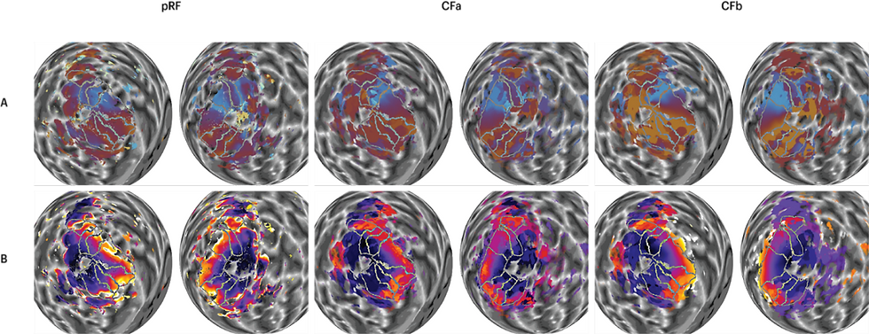
Figure 1: Visual field maps derived from the pRF and CF method. Polar angle maps (A) and eccentricity maps (B) on a spherical model of the two cortical hemispheres. Table of polar angle and eccentricity maps of a subject comparing the visual field maps derived from the pRF (left), CFa (middle) and CFb (right).

Fortunately, a novel technique called connective field (CF) modeling [6] has provided us with a promising method for visual field mapping and analysis, with fewer constraints than ever before. By using the same set of data, instead of determining the correlation between the largest brain response to a location in the visual field, CF modeling quantifies responses of the different brain regions that coincide with the responses in the primary visual cortex, which is also known as V1 [6]. Using a template of how the V1 represents the visual field, we can then translate the peak correlation in V1 into a prediction of other locations of the visual field that maps onto a given location in the brain. As the response is now identified in terms of the inter-areal activations rather than the correspondence between the position on the visual field and on our visual cortex, this method can theoretically liberate us from the previous requirements of steady fixation and controlled stimuli. Instead, subjects can freely view movies and naturally move or even close their eyes [7]. The subject's activity measured inside their V1 should thus yield adequate information necessary for retinotopic mapping.

During the summer, Assoc. Prof. Sam Schwarzkopf and I conducted research to assess the quality of the retinotopic maps derived from the CF method. We used the fMRI data previously collected from 25 subjects by Dr. Catherine Morgan and Prof. Steven Dakin. First, we analysed the data using the conventional pRF method. Then, we delineated the visual regions from both hemispheres of all the subjects using SamSrf software (visual field maps delineation can simply be understood as the tracing of the visual area borders based on the fMRI renders). The delineated regions were later also applied to the maps generated by the CF method. After that, we compared the pRF and CF map side-by-side, and qualitatively analysed the similarities and differences between the two methods. What happened after our first qualitative analysis was that we recognised that there were a few constraints that came with our original CF map derived from a group average template (hereafter referred to as CFa), so we included another CF template based on the probabilistic prediction of the cortical anatomy alone (hereafter referred to as CFb) [8]. Ultimately, we carried out statistical inference to investigate the difference between these three maps (pRF, CFa, and CFb) in terms of their coverage (the proportion of vertices in the occipital lobe that passed R2 > 0.01 threshold), angular and eccentricity1 correlation, and similarity (quantified by the mean Euclidean distance between pRFs in the maps).

Our Results

We first began with the qualitative analysis of the data. Initially, we compared the CFa map and pRF map side-by-side. Figure 1 shows example maps of a subject. Here, we summarise our observations between the maps derived from the two methods. Firstly, the CFa map appears to have greater coverage than the pRF map. This is particularly true in higher visual areas such as the V3B, LO, and MT. However, CF maps are generally cruder than the pRF maps, especially as pRF represents polar angle and eccentricity with smoother gradients. For polar angle, this means that maps based on CF (with either template) would be harder to delineate. Not only are the CF maps overall cruder, the borders of V2 and V3 in the CF maps appear to be clearer in dorsal (lower) areas, but less noticeable in the ventral (upper) areas. Borders of other areas such as V3A, V3B, and V4 also appear to be much weaker in the CF maps. For eccentricity maps, CFa appears to show a reversal around the medial borders where the peripheral edge should be with maximum eccentricity being lower than in the pRF maps. This is because of a statistical artefact when using a group average. The idea here is that, as the template is based on the group average, the mapping of eccentricity beyond the group average tends to be restricted. The probabilistic template used for CFb maps can thus overcome this issue.

Figure 2: Statistical analyses. Statistical tests were run to assess differences between the analyses for all vertices that passed the threshold of R2 > 0.01 and separately for each visual area, V1-V3B. (A) Friedman’s analysis of variance testing the difference between the coverage between the three analyses — pRF, CFa and CFb. (B) The Euclidean 4 distance between the pRFs in the pRF map and the CFa and CFb maps, respectively. Plots comparing the difference between the z-converted eccentricity (C) and polar (D) correlation between the pRF map and the CFa and CFb maps, respectively. *** p<0.001, ** p<0.01, * p<0.05

Next, we quantified the differences between the groups in terms of coverage, polar/angular correlation, eccentricity correlation, and the Euclidean distance. We wanted to be sure that any differences noticed in the qualitative analysis weren't due to our own subjective judgement. The results are shown in Figure 2. To assess the coverage differences between three groups (Figure 2A), we conducted a non-parametric ANOVA. We found that coverage for pRF maps was significantly lower than for CF maps. This difference was observed across all vertices (the data points across the brain template) that passed the set threshold, as well as separately in all individual regions. To put it another way, we found that there are differences in map coverage between the two methods, with pRF coverage being significantly lower than the CF. The results here agree very well with the qualitative analysis we conducted.

Next, we compared the CFa and CFb maps to the pRF map; this assumes that the pRF constitutes something of a ground truth for the best possible map that can be obtained for this data. Comparing the correlation between the pRF polar angle estimates (Figure 2D) and those in the two CF maps using a paired t-test showed a significantly stronger correlation for CFa across all vertices and in regions such as V1, V2, V3, and V3B. The results indicate that CFa polar angle maps correlate better with the pRF map than the CFb maps. Despite the CFb template being smoother, CFb polar angle maps lack details and are very crude. This means that on several occasions, polar reversals displayed on CFb are represented by large patches of polar angle reversal with a lack of precise location. Meanwhile, the CFa maps are also cruder than the pRF map, but the locations of polar reversals resemble the conventional pRF map better.

In contrast, we found a significantly stronger correlation between pRF eccentricity (Figure 2C) and the CFb eccentricity in all vertices, and in individual regions such as V1, V2, and V3. This means that the CFb template is more closely correlated to the pRF maps when it comes to the eccentricity mapping. The better correlation found in CFb may be attributed to the template covering the full 90 degrees eccentricity [8], while the CFa template is constrained by the 10 degrees limit of the stimulation screen in the scanner. Since CFa is based on a group average, it contains a statistical artefact manifesting as an eccentricity reversal. As CFb does not pose the same constraints, the eccentricity maps no longer display reversals on the peripheral edge of the visual cortical regions. This therefore becomes more consistent with the conventional pRF eccentricity mapping.

We further investigated the map similarity quantified by the mean Euclidean distance between the position of pRFs and CFs in each map (Figure 2B). Euclidean distances were significantly larger for CFb maps across all vertices and in all individual regions. This indicates that CFb maps captured pRF positions less accurately. That is to say, the CFa maps are overall more similar to the pRF map than the CFb maps.

Future Implications

The current research suggests that the new method of retinotopic mapping can open a window of opportunities. It can help us achieve new ways of testing and research we couldn't have previously done. Conventional visual field mapping studies are prone to several confounds. The prolonged fixation required in the study can pose several problems for studying a wide range of the population. The subject's ability to move their eyes freely is crucial for those with visual disorders such as amblyopia [9] and nystagmus (involuntary repetitive movement of the eyes), and those with other ocular or neurological pathologies. Thus, the new method may provide robustness in the presence of eye movements or a blurred and obstructed visual image [9-10]. Taken together, the method has potential for revealing new insights about visual cortical organisation in various pathologies, as well as in healthy participants at the extremes of the human lifespan.

Another promising implication that this research may lead to is mapping human peripheral vision. Due to several factors, such as the fixation and technological limitations, retinotopic mapping of the human periphery has thus far been considered difficult, or even impossible. The stimulus typically used for conventional retinotopic mapping is often very small, insufficient, and presented near the centre of gaze; therefore, they cannot produce a response in the periphery. The CF method permits movie watching and free eye movements. Thus, it allows the subjects to explore their entire visual field rather than fixating on a single spot [7]. With free eye movements, we can now ensure that the subject's eye movements cover the whole visual field, including the far periphery. Moreover, it enables researchers to use more engaging and interesting stimuli than what was used in conventional pRF mapping experiments, thus helping enhance the participant’s motivation, and improve data quality.

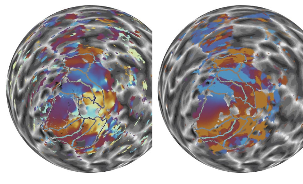
Figure 3: Polar angle maps. Side-by-side comparison between the right hemisphere pRF (right) and the CFb polar angle maps (left).

Retinotopic mapping with connective field modeling is relatively new, and there are yet to be many studies on the topic. This is the first comprehensive comparison that assesses the quality of retinotopic maps generated by the connective field modeling method. Our results show that there is still substantial room for improvement for this cutting-edge methodology. The results from the current study will help us point towards methodological improvements. We have already begun work on a new approach: while our analysis shown here determined the peak correlation between the position in the visual field and the voxel response to determine the predicted pRF coordinates, our new approach does the opposite. It uses the predicted pRF coordinates from the template to project the correlations into visual space, and then fits a pRF to those correlations in visual space. In addition to estimating pRF position, this approach therefore also estimates pRF size. Moreover, it frees the CF analysis from the constraint that it needs to be conducted separately in each cortical hemisphere. Once we test these improvements, the next step we intend to do is to quantify the hypothetical robustness of this new CF map in the presence of eye movements.

References

1. B. A. Wandell, S. O. Dumoulin, and A. A. Brewer, “Visual field maps in human cortex.,” vol. 56, no. 2, pp. 366–383, 2007, doi: 10.1016/j.neuron.2007.10.012. https://pubmed.ncbi.nlm.nih.gov/23684878/

2. S. O. Dumoulin and B. A. Wandell, “Population receptive field estimates in human visual cortex,” 2007, doi: 10.1016/j.neuroimage.2007.09.034. [Online]. Available: www.elsevier.com/locate/ynimg

3. S. Lee, A. Papanikolaou, N. K. Logothetis, S. M. Smirnakis, and G. A. Keliris, “A new method for estimating population receptive field topography in visual cortex,” vol. 81, pp. 144–157, Nov. 2013, doi: 10.1016/J.NEUROIMAGE.2013.05.026. [Online]. Available: https://pubmed.ncbi.nlm.nih.gov/23684878/

4. M. Farahbakhsh et al., “A demonstration of cone function plasticity after gene therapy in achromatopsia,” p. 2020.12.16.20246710, Oct. 2021, doi: 10.1101/2020.12.16.20246710. [Online]. Available: https://www.medrxiv.org/content/10.1101/2020.12.16.20246710v2

5. V. K. Tailor, D. S. Schwarzkopf, and A. H. Dahlmann-Noor, “Neuroplasticity and amblyopia: Vision at the balance point,” vol. 30, no. 1, pp. 74–83, 2017, doi: 10.1097/WCO.0000000000000413.

6. K. V. Haak et al., “Connective field modeling,” vol. 66, pp. 376–384, Feb. 2013, doi: 10.1016/J.NEUROIMAGE.2012.10.037. [Online]. Available: https://pubmed.ncbi.nlm.nih.gov/23110879/

7. T. Knapen, “Topographic connectivity reveals task-dependent retinotopic processing throughout the human brain,” vol. 118, no. 2, Jan. 2021, doi: 10.1073/PNAS.2017032118/-/DCSUPPLEMENTAL. [Online]. Available: https://www.pnas.org/content/118/2/e2017032118

8. N. C. Benson, O. H. Butt, R. Datta, P. D. Radoeva, D. H. Brainard, and G. K. Aguirre, “The retinotopic organization of striate cortex is well predicted by surface topology,” vol. 22, no. 21, pp. 2081–2085, Nov. 2012, doi: 10.1016/J.CUB.2012.09.014. [Online]. Available: https://pubmed.ncbi.nlm.nih.gov/23041195/

9. S. Clavagnier, S. O. Dumoulin, and R. F. Hess, “Is the Cortical Deficit in Amblyopia Due to Reduced Cortical Magnification, Loss of Neural Resolution, or Neural Disorganization?,” vol. 35, no. 44, p. 14740, Nov. 2015, doi: 10.1523/JNEUROSCI.1101-15.2015. [Online]. Available: /pmc/articles/PMC6605231/

10. B. Barton and A. A. Brewer, “fMRI of the rod scotoma elucidates cortical rod pathways and implications for lesion measurements,” vol. 112, no. 16, pp. 5201–5206, Apr. 2015, doi: 10.1073/PNAS.1423673112/-/DCSUPPLEMENTAL. [Online]. Available: https://www.pnas.org/content/112/16/5201